Nerds
Note
Please make sure that you have completed the Introduction to Regression in R module on Data Camp before going through this.
Take This
First things first, please go and take the Nerdy Personality Attributes Scale.
Read Up
Please make sure that you have read the paper An exploratory factor analysis of the Nerdy Personality Attributes Scale in a sample of self-identified nerds/geeks (Finister, Pollet, & Neave, 2020) included in this week’s downloads.
Data Files
Please download the files we’ll need.
Prerequisites
Like last week, open up Rstudio and create a new script by going to File > New File > R Script. Save this in an easily accessible folder. Now unzip this week’s data set and take the files that start with Nerdy and end a .csv - and drop them all in a folder of their own.
Before we load the libraries, we’re going to grab three packages called mice and naniar that are on CRAN. To install them, please run the following command in your console
install.packages(c("mice", "naniar"), dependencies = TRUE)
or you can simply use the dropdown menu by going to Tools > Install Packages and type in mice, naniar or mice naniar. Remember to have Install dependencies checkmarked!
If you would like to know more about the mice package and/or the concept of imputation, take a look at the Flexibile Imputation of Missing Data site.
Now please go ahead and load up the following libraries or download and load if needed
library("tidyverse")
library("mice")
library("naniar")
library("reactable")
Then set the working directory to the location of the script by running
setwd(dirname(rstudioapi::getActiveDocumentContext()$path))
in your console or by selecting Session > Set Working Directory > To Source File Location.
Data Files
We’ll be looking at responses from a subsample of 10 from 25442 people who took this test.
Loading a Local Data Set
If you remember how to load a local dataset, then please skip this section
nerdy_data <-
  read_csv("NerdyDataMissing.csv")
## Rows: 10 Columns: 26
## ── Column specification ────────────────────────────────────────────────────────
## Delimiter: ","
## dbl (26): Q1, Q2, Q3, Q4, Q5, Q6, Q7, Q8, Q9, Q10, Q11, Q12, Q13, Q14, Q15, ...
##
## ℹ Use `spec()` to retrieve the full column specification for this data.
## ℹ Specify the column types or set `show_col_types = FALSE` to quiet this message.
nerdy_pm_codebook <-
  read_csv("NerdyCodebook_PM.csv")
## Rows: 26 Columns: 2
## ── Column specification ────────────────────────────────────────────────────────
## Delimiter: ","
## chr (2): Index, Item
##
## ℹ Use `spec()` to retrieve the full column specification for this data.
## ℹ Specify the column types or set `show_col_types = FALSE` to quiet this message.
nerdy_pm_measures <-
  read_csv("NerdyMeasures_PM.csv")
## Rows: 5 Columns: 2
## ── Column specification ────────────────────────────────────────────────────────
## Delimiter: ","
## chr (1): Description
## dbl (1): Measure
##
## ℹ Use `spec()` to retrieve the full column specification for this data.
## ℹ Specify the column types or set `show_col_types = FALSE` to quiet this message.
and take a look at the data
nerdy_data %>%
  head()
## # A tibble: 6 × 26
##      Q1    Q2    Q3    Q4    Q5    Q6    Q7    Q8    Q9   Q10   Q11   Q12   Q13
##   <dbl> <dbl> <dbl> <dbl> <dbl> <dbl> <dbl> <dbl> <dbl> <dbl> <dbl> <dbl> <dbl>
## 1     3     5     3     3     5     5     5    NA    NA     5     4     5     5
## 2    NA    NA     4     3     5    NA     5     1     4    NA     1    NA     4
## 3     5    NA     5     5     5    NA     5     5     5     5     5     4     5
## 4    NA     5    NA     5     5    NA     5    NA     5     5     5    NA     4
## 5     4    NA    NA     4    NA     4    NA     4     4     5     4     4    NA
## 6     4     4     4     4     4     4     5     3    NA    NA     4     4     3
## # … with 13 more variables: Q14 <dbl>, Q15 <dbl>, Q16 <dbl>, Q17 <dbl>,
## #   Q18 <dbl>, Q19 <dbl>, Q20 <dbl>, Q21 <dbl>, Q22 <dbl>, Q23 <dbl>,
## #   Q24 <dbl>, Q25 <dbl>, Q26 <dbl>
or via the reactable() package1
reactable(nerdy_data,
          defaultPageSize = 5,
          showPageSizeOptions = TRUE)
as well as the codebook and measures
nerdy_pm_codebook
## # A tibble: 26 × 2
##    Index Item
##    <chr> <chr>
##  1 Q1    I am interested in science.
##  2 Q2    I was in advanced classes.
##  3 Q3    I like to play RPGs. (Ex. D&D)
##  4 Q4    My appearance is not as important as my intelligence.
##  5 Q5    I collect books.
##  6 Q6    I prefer academic success to social success.
##  7 Q7    I watch science related shows.
##  8 Q8    I spend recreational time researching topics others might find dry or …
##  9 Q9    I like science fiction.
## 10 Q10   I would rather read a book than go to a party.
## # … with 16 more rows
nerdy_pm_measures
## # A tibble: 5 × 2
##   Measure Description
##     <dbl> <chr>
## 1       5 Agree
## 2       4 Somewhat Agree
## 3       3 Neutral
## 4       2 Somewhat Disagree
## 5       1 Disagree
Missingness
You may be asking why should I care about missing data? and can’t I just delete them? Great questions!
Some analyses like linear regression that you covered this week require complete observations, but still in most statistical software you won’t get an error when feeding the system with data containing missing values (cough cough but R does tell you there’s an error cough cough).
Instead, most non R softwares automatically delete incomplete cases…and silently at that which is pretty rude. However, if you plan to say make conclusions about the entire data set. an interpretation just wouldn’t be appropriate since you cannot guarantee the same observations. Even worse, by dropping the observations completely we lose statistical power which in a nutshell results in a likelihood that you’ll conclude that there isn’t an effect when there is (aka a Type II error). Oh but it gets even better, the dropped observations could provide crucial information about the problem of interest resulting in biased results.
In practice, this can be the difference between being able to conclude a treatment likely works and reporting maybe something happened but we don’t know. So missing data is a big problem that we still haven’t been able to tackle directly yet2.
To tackle this issue, there are two prevailing philosophical approaches. On one side are those who believe that the data is what it is and you have to deal with what you get. On the other side you have those that believe a machine, whether it be using an algorithm by itself or coupled with artificial intelligence, can predict the likely values that should have been there given certain assumptions are met (which we cover in the next section)3.
So for the latter group, there are a number of tactics that can be used to tackle this missingness issue, but the main three are
pairwise deletion: a method in which data for a variable pertinent to a specific assessment are included, even if values for the same individual on other variables are missing.
listwise deletion: a method in which an entire case record is excluded from statistical analysis if values are found to be missing for any variable of interest.
imputation: a procedure for filling in missing values in a data set before analyzing the resultant completed data set.
Most people in this camp use the deletion techniques as a last resort because there is wariness about removing data. In this walkthrough, we’ll cover the last approach: imputation.
Note
Please be aware that this idea of addressing missingness in a data set is a multifaceted issue, there is a lot that is not covered here, and in practice it is very easy to go down a rabbit hole. This walkthrough is written in a way that hopefully brings a high level topic down to an understandable level. In doing that, some information is lost or has been set aside for the sake of simplicity. With that said, view this through the lens of a problem that you might or will even likely come across. The issue is that few people know what to do about missing data so they either ignore or delete it without considering the ramifications. However if you are interested in learning more or need clarifications, please reach out!
Assumptions
If you have taken statistics in the past, then you likely know about these things called assumptions, or criteria that have to be satisfied before running a statistical test (e.g. t-test, ANOVA, etc.). This is also true when dealing with missing data points, in that we have to determine if our data is
| Type | Shorthand | Description | Traits | What Can You Do? |
|---|---|---|---|---|
| Missing Completely At Random | MCAR | The locations of missing values are random and not dependent on other data. | Strong assumptions; difficult or possibly impossible to detect | Deletion techniques or imputation with confidence in reporting |
| Missing At Random | MAR | The locations of missing values are random BUT depend on some other observed data | Neutral(ish) assumptions; possible to detect | Advanced imputation with caution in reporting. |
| Missing Not At Random | MNAR | There is a pattern to the missing values | Weak assumptions; easy to detect | An inability to report anything meaningful (get new or more data because this is bad). |
What to Do About Missing Data
In the real world, data involving humans is rarely results in a complete set of values. As you can imagine, this is nearly always the case when conducting surveys where respondents are free to skip questions4. So what can you do?
Testing for MCAR
While it is difficult, if not impossible to figure out if a dataset is MCAR, we can use probability to determine if it could be. The best way to do this is to figure out a formula for the regression, and to test that - but we’re not going to take that approach given the makeup of the course. A simpler, yet less robust way is to use a technique developed by Little (1988) that basically gives is a probability that a data set is MCAR. But remember, there is always an associated probability that it may not be too!
Using the narniar package, we can use the test. In a callback to your introductory statistics course, the null hypothesis ($H_0$) is that the data is MCAR while the test statistic is a chi-squared ($\chi^2$) value.
mcar_test(nerdy_data)
## # A tibble: 1 × 4
##   statistic    df p.value missing.patterns
##       <dbl> <dbl>   <dbl>            <int>
## 1      90.0   169    1.00               10
Given the high \(p\)-value, we can say that nerdy_data could be MCAR. To get an idea of the number of items that have missing values, you can use
n_var_miss(nerdy_data)
## [1] 26
To view the missingness by item, we can use the following
gg_miss_var(nerdy_data) +
  guides(color = "none")
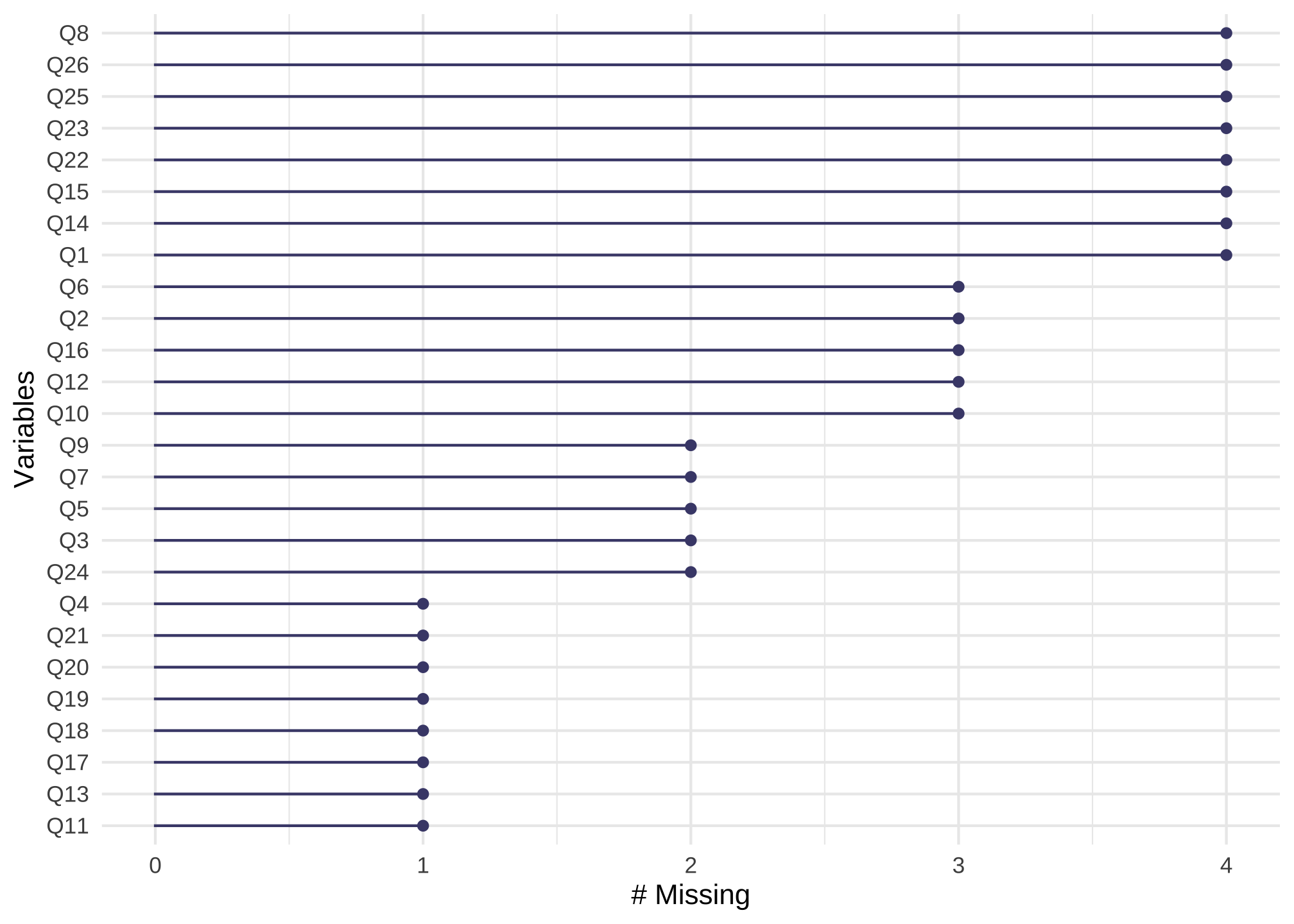
which just says all 26 columns have at least one missing value. To see common missingness by items, we can use
gg_miss_upset(nerdy_data,
              nsets = n_var_miss(nerdy_data))
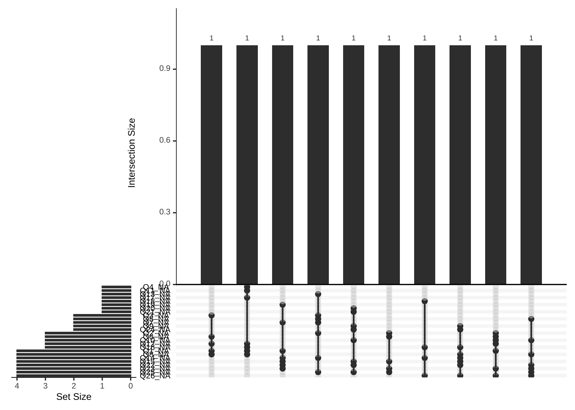
where nsets are the number of columns which shows us
- all of the variables with missing values
- all of the common values that are missing
- each combination of missing values occurs once
but that is really difficult to read and we’re just getting a feel for the missingness, so let’s try limiting the number of variables to say the top 5
gg_miss_upset(nerdy_data,
              nsets = 5)
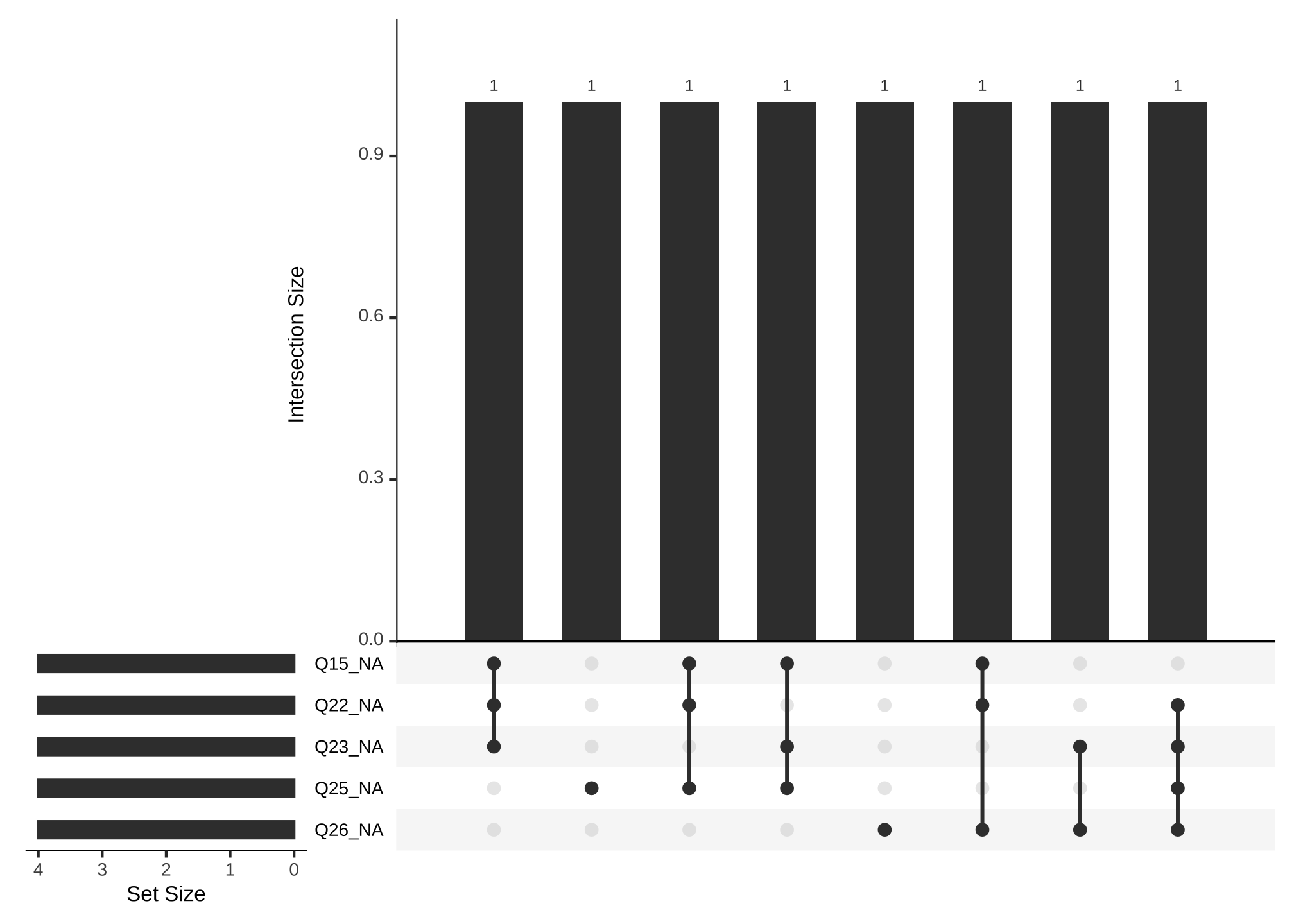
OK that’s better! Now its easier to see questions 15, 22, and 23 share a common missing value and so forth.
We can even use ggplot to visualize this differently by item. First we have to add a column for the respondents by
nerdy_data_rowid <-
  nerdy_data %>%
  rowid_to_column("respondent")
which just adds a column in front with unique ids.
nerdy_data_rowid
## # A tibble: 10 × 27
##    respondent    Q1    Q2    Q3    Q4    Q5    Q6    Q7    Q8    Q9   Q10   Q11
##         <int> <dbl> <dbl> <dbl> <dbl> <dbl> <dbl> <dbl> <dbl> <dbl> <dbl> <dbl>
##  1          1     3     5     3     3     5     5     5    NA    NA     5     4
##  2          2    NA    NA     4     3     5    NA     5     1     4    NA     1
##  3          3     5    NA     5     5     5    NA     5     5     5     5     5
##  4          4    NA     5    NA     5     5    NA     5    NA     5     5     5
##  5          5     4    NA    NA     4    NA     4    NA     4     4     5     4
##  6          6     4     4     4     4     4     4     5     3    NA    NA     4
##  7          7     5     3     4     3    NA     4     4    NA     5    NA     3
##  8          8    NA     3     4     5     5     3    NA     5     3     5     4
##  9          9    NA     5     5    NA     2     3     0    NA     4     4    NA
## 10         10     4     5     5     5     4     3     5     4     4     5     1
## # … with 15 more variables: Q12 <dbl>, Q13 <dbl>, Q14 <dbl>, Q15 <dbl>,
## #   Q16 <dbl>, Q17 <dbl>, Q18 <dbl>, Q19 <dbl>, Q20 <dbl>, Q21 <dbl>,
## #   Q22 <dbl>, Q23 <dbl>, Q24 <dbl>, Q25 <dbl>, Q26 <dbl>
And then let’s visualize it for Q1
ggplot(data = nerdy_data_rowid,
       aes(x = respondent,
       y = Q1)) +
  geom_miss_point()
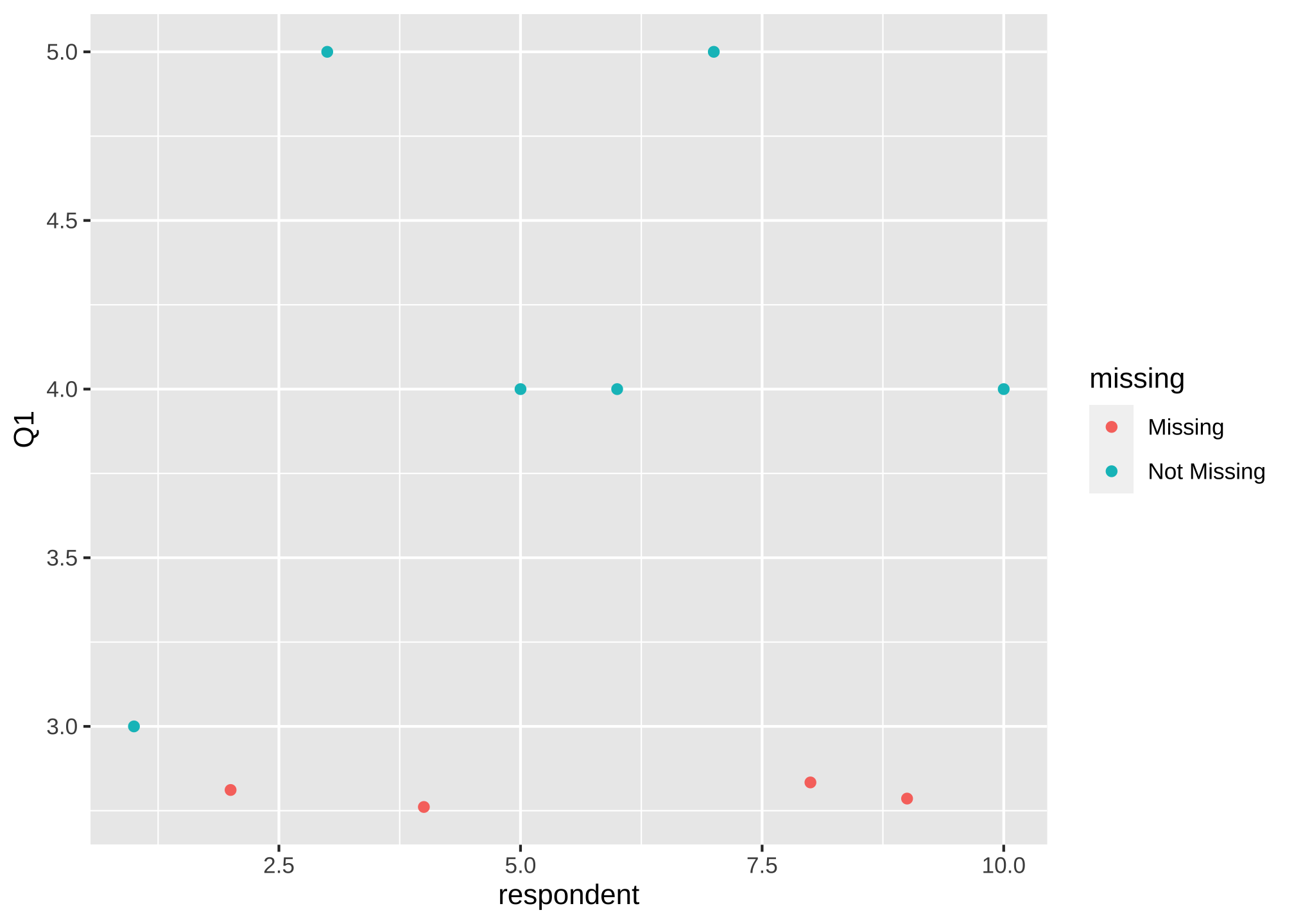
or maybe its easier without the default grey background and bigger
ggplot(data = nerdy_data_rowid,
       aes(x = respondent,
       y = Q1)) +
  geom_miss_point(size = 2) +
  theme_minimal()
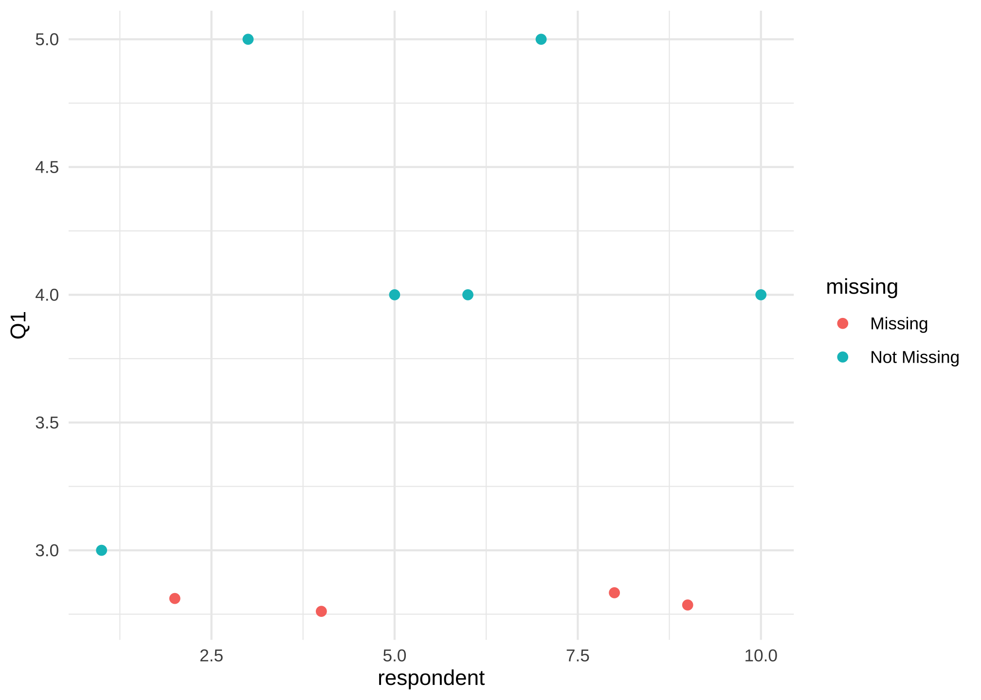
On a side note, yes the x-axis looks odd and we could fix it, but we’re just exploring.
Multiple Imputation
Run the command mice() from the aptly named mice package to impute a data set. Here m is the number of times your computer applies the imputation algorithm to the data set
nerdy_data_imputed <-
  mice(nerdy_data,
       m = 15,
       method = 'pmm')  %>%
  complete(1) %>%
  as_tibble()
## Warning: Number of logged events: 3448
nerdy_data_imputed
## # A tibble: 10 × 26
##       Q1    Q2    Q3    Q4    Q5    Q6    Q7    Q8    Q9   Q10   Q11   Q12   Q13
##    <dbl> <dbl> <dbl> <dbl> <dbl> <dbl> <dbl> <dbl> <dbl> <dbl> <dbl> <dbl> <dbl>
##  1     3     5     3     3     5     5     5     3     4     5     4     5     5
##  2    NA     4     4     3     5     5     5     1     4    NA     1     5     4
##  3     5     5     5     5     5     5     5     5     5     5     5     4     5
##  4    NA     5     4     5     5     3     5     4     5     5     5     4     4
##  5     4     5     5     4     4     4     5     4     4     5     4     4     5
##  6     4     4     4     4     4     4     5     3     3    NA     4     4     3
##  7     5     3     4     3     4     4     4     3     5    NA     3     3     4
##  8    NA     3     4     5     5     3     4     5     3     5     4     4     3
##  9    NA     5     5     4     2     3     0     4     4     4     1     4     5
## 10     4     5     5     5     4     3     5     4     4     5     1     4     4
## # … with 13 more variables: Q14 <dbl>, Q15 <dbl>, Q16 <dbl>, Q17 <dbl>,
## #   Q18 <dbl>, Q19 <dbl>, Q20 <dbl>, Q21 <dbl>, Q22 <dbl>, Q23 <dbl>,
## #   Q24 <dbl>, Q25 <dbl>, Q26 <dbl>
Now there are a lot of ways to impute data, some which will do a better job than others and dependent of what type of data you have. To see a list, just run ?mice::mice and scroll about halfway down the help page. You can change the approach by replacing pmm in method = 'pmm' above.
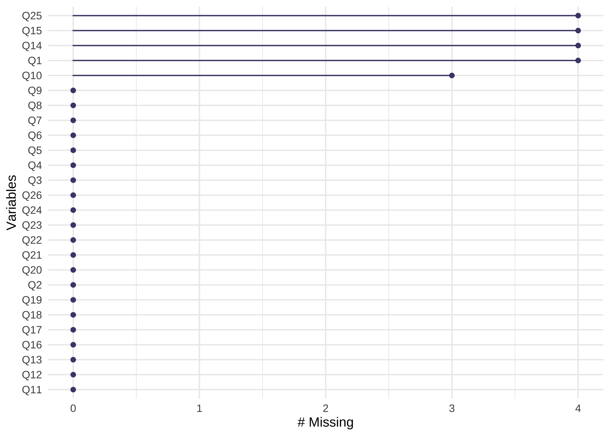
Anyway is our new data set any better because it look like there are still missing values. Well let’s take a look
n_var_miss(nerdy_data_imputed)
## [1] 5
gg_miss_var(nerdy_data_imputed) +
  guides(color = "none")
gg_miss_upset(nerdy_data_imputed)
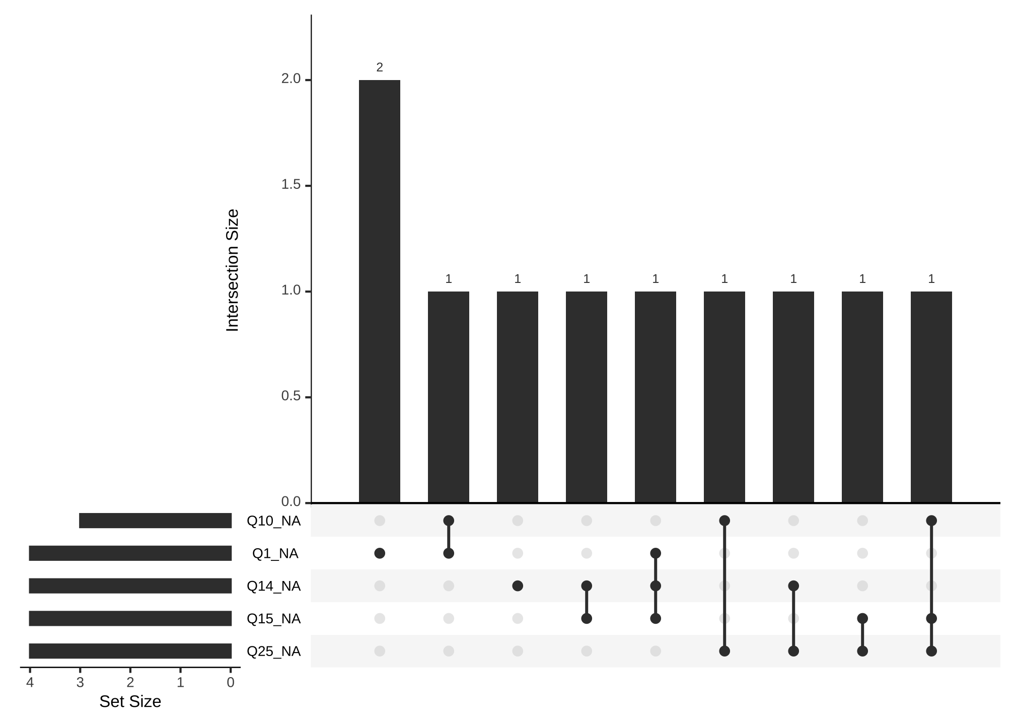
Oh that looks a lot better! We could change m or the method to get a more complete data set.
The Data
I randomized missing data the original subset which can be seen by opening the NerdyDataSubset.csv file. To take a look at the original full data, take a look at NerdyDataFull.csv. The remaining files address measures and data from that set.
More About the Packages
The
narianpackage has alot of functionality not covered here. Take a look at the following for more helpThe
micepackage is confusing at times and can hurt your head, but its by far one of the most versatile and powerful packages to impute data. So if you find yourself with missing data, it may be beneficial to dive in headfirst. To get acquainted, a couple vignettes can be found using the link below
Scroll to the right to see all columns ↩︎
…though recent advances in machine learning have brought us closer in the past three years than we have had in the past 50 ↩︎
In all fairness, I am in this group and absolutely biased. ↩︎
You’re first reaction may be to require respondents to address items -aka a forced response- but that almost always backfires resulting in a higher rate of nonresponses ↩︎